Capítulo 9 Tareas
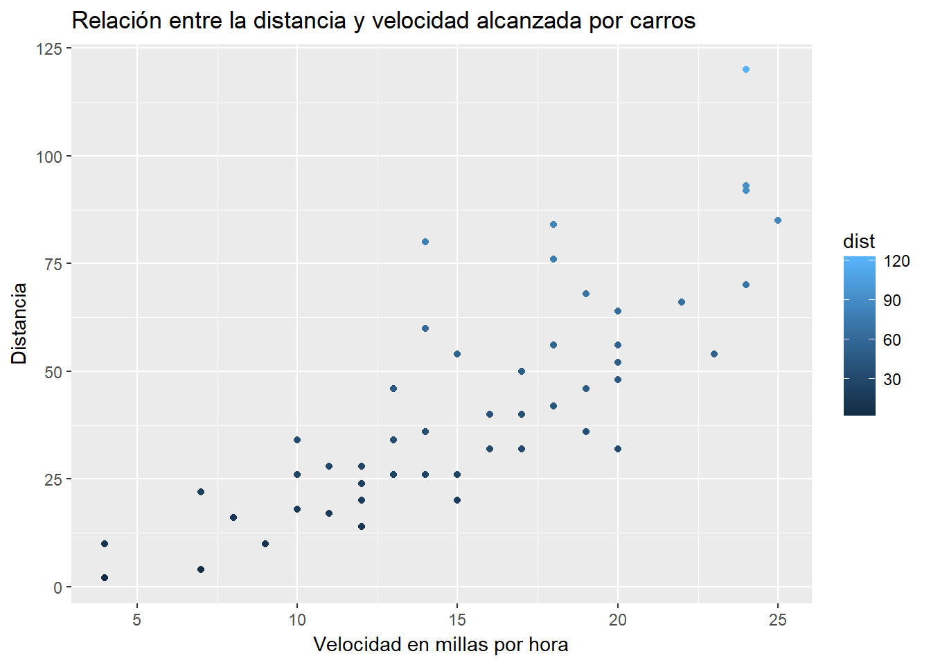
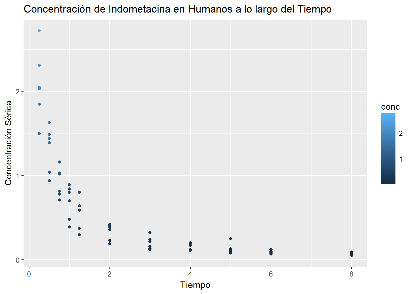
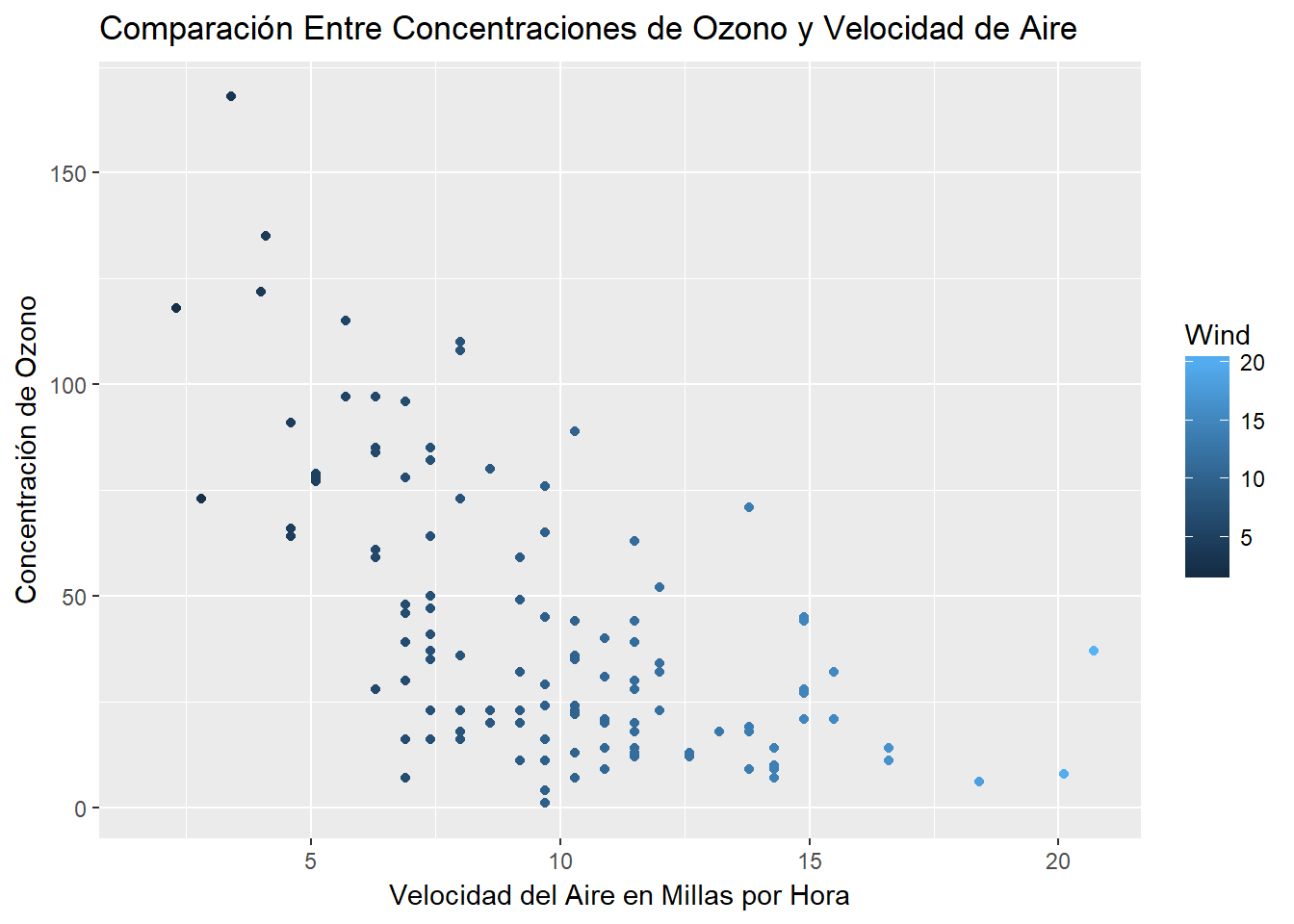
9.1 Point Chart
9.2 Stratified Sampling
author: Dolores Ojeda, Gener Avilés R date: 2017-03-05
9.2.1 What is Stratified Sampling?
Population is partitioned in non-overlaping groups, called strata and a sample is collected from each stratum following a determined design.
9.2.2 Why use Stratified Sampling?
- May produce smaller error when estimating than simple random sample. Specially when measurements within strata have realitve small variation. - Cost by observation reduced. - There may be a need to have a subgroup (stratum) with similar estimates of those of the population.
9.2.3 Example
The Titanic Database:
##      pclass         survived         name               sex
##  Min.   :1.000   Min.   :0.000   Length:1310        Length:1310
##  1st Qu.:2.000   1st Qu.:0.000   Class :character   Class :character
##  Median :3.000   Median :0.000   Mode  :character   Mode  :character
##  Mean   :2.295   Mean   :0.382
##  3rd Qu.:3.000   3rd Qu.:1.000
##  Max.   :3.000   Max.   :1.000
##  NA's   :1       NA's   :1
##       age              sibsp            parch          ticket
##  Min.   : 0.1667   Min.   :0.0000   Min.   :0.000   Length:1310
##  1st Qu.:21.0000   1st Qu.:0.0000   1st Qu.:0.000   Class :character
##  Median :28.0000   Median :0.0000   Median :0.000   Mode  :character
##  Mean   :29.8811   Mean   :0.4989   Mean   :0.385
##  3rd Qu.:39.0000   3rd Qu.:1.0000   3rd Qu.:0.000
##  Max.   :80.0000   Max.   :8.0000   Max.   :9.000
##  NA's   :264       NA's   :1        NA's   :1
##       fare            cabin             embarked
##  Min.   :  0.000   Length:1310        Length:1310
##  1st Qu.:  7.896   Class :character   Class :character
##  Median : 14.454   Mode  :character   Mode  :character
##  Mean   : 33.295
##  3rd Qu.: 31.275
##  Max.   :512.329
##  NA's   :2
##      boat                body        home.dest
##  Length:1310        Min.   :  1.0   Length:1310
##  Class :character   1st Qu.: 72.0   Class :character
##  Mode  :character   Median :155.0   Mode  :character
##                     Mean   :160.8
##                     3rd Qu.:256.0
##                     Max.   :328.0
##                     NA's   :1189
9.2.3.1 Variable Codes
- Pclass: 1 = Upper, 2 = Middle, 3 = Lower. - SibSp: Number of Siblings/Spouses aboard. - Parch: Number of Parents/Children Aboard. - Embarked: C = Cherbourg, Q = Queenstown, S = Southampton.
9.2.3.2 Calculating Probabilities to select people who embarked in Queenstown
\(P(A) = \frac{\text{Numero de elementos de A}}{n}\)
There are 1310 entries, and 123 of them embarked in Queenstown, nevertheless the risk of dying was equally present for them as for the passengers from Southampton or Cherbourg.
If a uniform proability is calculated the numbers are:
- \(P(Q) = \frac{123}{1310} =\) 0.0938931 - \(P(C) = \frac{270}{1310} =\) 0.2061069 - \(P(S)\frac{914}{1310} =\) 0.6977099
This approximation will hinder the process of data mining and, eventually, the generation of a machine learning model for survival prediction.
9.2.3.3 Fixing the Problem
By using stratified sampling we can raise the probability for the group that boarded in Queenstown and survived to be selected, therefore, taken in consideration for the generation of a survival prediction model. For this we will use conditional probability:
\(P(Survived|EmbarkedQ)= \frac{P(Survived\cap EmbarkedQ)}{P(EmbarkedQ)} = \frac{44}{123}=\) 0.3577236
library(dplyr)
Q<-filter(titanic, embarked == "Q" & survived == 1)
count(Q)
## # A tibble: 1 x 1
## n
## <int>
## 1 44Carlos Pérez-González, Marcos Colebrook-Santamaría. 2014. “Curso Introductorio de R: Introducción a La Interfaz de Rstudio.” http://mcolebrook.github.io/CursoRStudio/RStudio.html#(1).
Chambers, John. 2000. “Stages in the Evolution of S.” March. http://ect.bell-labs.com/sl/S/history.html.
Data, and Story Library. n.d. “Cereals Data Set.” http://lib.stat.cmu.edu/DASL/Datafiles/Cereals.html.
Leek, Jeff. 2016. “How to Share Data with a Statistician.” November. https://github.com/jtleek/datasharing.
López, Francisco Javier Barón. 2013. “Apuntes Y Vídeos de Bioestadística.” https://www.bioestadistica.uma.es/baron/apuntes/.